基于Keras解决深度学习中的回归问题

公众号：尤而小屋
作者：Peter
编辑：Peter

持续更新《Python深度学习》一书的精华内容，仅作为学习笔记分享。

本文是第4篇：基于Keras解决深度学习中的回归问题。

Keras内置数据集

回归问题中使用的是内置的波士顿房价数据集。在keras中有多个内置的数据集：

• 波士顿房价数据集
• CIFAR10数据集（包含10种类别的图片集）
• CIFAR100数据集（包含100种类别的图片集）
• MNIST数据集（手写数字图片集）
• Fashion-MNIST数据集（10种时尚类别的图片集）
• IMDB电影点评数据集
• 路透社新闻数据集

其中IMDB数据集在二分类问题中被使用过，路透社新闻数据集在多分类问题中被使用。

In [1]:

import numpy as np
np.random.seed(1234)  # 设置随机种子

import matplotlib.pyplot as plt
%matplotlib inline

import warnings 
warnings.filterwarnings("ignore")  # 忽略notebook中的警告

导入数据

In [2]:

from  keras.datasets import boston_housing

(train_data,train_targets), (test_data, test_targets) = boston_housing.load_data()  

查看数据的基本信息：

In [3]:

train_data[:3]

Out[3]:

array([[1.23247e+00, 0.00000e+00, 8.14000e+00, 0.00000e+00, 5.38000e-01,
        6.14200e+00, 9.17000e+01, 3.97690e+00, 4.00000e+00, 3.07000e+02,
        2.10000e+01, 3.96900e+02, 1.87200e+01],
       [2.17700e-02, 8.25000e+01, 2.03000e+00, 0.00000e+00, 4.15000e-01,
        7.61000e+00, 1.57000e+01, 6.27000e+00, 2.00000e+00, 3.48000e+02,
        1.47000e+01, 3.95380e+02, 3.11000e+00],
       [4.89822e+00, 0.00000e+00, 1.81000e+01, 0.00000e+00, 6.31000e-01,
        4.97000e+00, 1.00000e+02, 1.33250e+00, 2.40000e+01, 6.66000e+02,
        2.02000e+01, 3.75520e+02, 3.26000e+00]])

In [4]:

train_data.shape, test_data.shape

Out[4]:

((404, 13), (102, 13))

数据标准化

在机器学习中，对数据进行标准化是非常重要的，主要有以下原因：

• 消除量纲影响：不同特征的数值大小可能相差很大，例如重量和价格。如果这些特征之间具有很大的差异，那么某些特征的值可能会主导模型的训练过程，从而削弱其他特征的重要性。通过标准化，可以将所有特征的值缩放到相同的尺度上，消除量纲的影响。
• 加速收敛：在机器学习算法中，梯度下降是一种常用的优化算法。当数据存在较大的尺度差异时，梯度更新可能会变得非常慢，导致算法收敛速度变慢。通过标准化，可以减少尺度差异，从而加速梯度下降算法的收敛速度。
• 提高模型性能：标准化可以使数据分布更加均匀，避免出现极端值或离群点。这有助于提高模型的泛化能力和性能。 因此，对数据进行标准化是机器学习中一个重要的预处理步骤，可以提升模型的训练效果和预测性能。

首先求出训练集的均值和标准差，进行标准化；再使用训练集的均值和标准差对测试集进行标准化。

In [5]:

# 手动标准化

mean = train_data.mean(axis=0) # 均值
train_data -= mean

std = train_data.std(axis=0)
train_data /= std 

对测试集的标准化：

In [6]:

# 仍然使用训练集的mean std

test_data -= mean
test_data /= std

搭建网络

In [7]:

from keras import models, layers

In [8]:

def build_model():
    model = models.Sequential()
    # 输入层
    model.add(layers.Dense(64,activation="relu",input_shape=(train_data.shape[1],)))
    # 隐藏层
    model.add(layers.Dense(64,activation="relu"))
    # 输出层：回归问题预测一个值，最终只有一个单元
    model.add(layers.Dense(1))
    model.compile(optimizer="rmsprop",  # 优化器
                  loss="mse",   # 损失
                  metrics=["mae"])  # 评价指标
    return model

k折交叉验证

本小节的部分代码和原文有不同：

In [9]:

k = 5  # k折

num_val_samples = (len(train_data)) // k

num_epochs = 500

all_mae = []
all_val_mae = []
all_loss = []
all_val_loss = []

for i in range(k):
    
    print(f"第 {i+1} fold正在running")
    
    # 准备验证集数据
    valid_data = train_data[i*num_val_samples:(i+1)*num_val_samples]
    valid_targets = train_targets[i*num_val_samples:(i+1)*num_val_samples]
    
    # 准备训练集（除去验证集部分）
    part_train_data = np.concatenate([
        train_data[:i*num_val_samples],  # 索引i之前和i+1之后，两部分合并起来成为训练集
        train_data[(i+1)*num_val_samples:]
    ],axis=0)
    
    part_train_targets = np.concatenate([
        train_targets[:i*num_val_samples],
        train_targets[(i+1)*num_val_samples:]
    ],axis=0) 
    
    
    # 模型训练
    model = build_model()
    history = model.fit(part_train_data,
             part_train_targets,
             epochs=num_epochs,
             batch_size=1,
             verbose=0,   # 静默模式，不显示每个epochs的具体打印信息
             validation_data=[valid_data,valid_targets])
    history_dict = history.history
    
    mae = history_dict["mae"]  # 训练集的mae
    val_mae = history_dict["val_mae"]  # 训练集的mae
    loss = history_dict["loss"]
    val_loss = history_dict["val_loss"]
    
    all_mae.append(mae)
    all_val_mae.append(val_mae)
    all_loss.append(loss)
    all_val_loss.append(val_loss)
第 1 fold正在running
第 2 fold正在running
第 3 fold正在running
第 4 fold正在running
第 5 fold正在running

模型指标可视化

In [10]:

len(all_mae) # 5折

Out[10]:

5

In [11]:

# all_mae[0]  # 第1折的全部信息

第1折有500个元素(epochs=500)

In [12]:

len(all_mae[0])

Out[12]:

500

计算每个指标的平均值：

In [13]:

mae_average = [np.mean([x[i] for x in all_mae]) for i in range(num_epochs)]
mae_val_average = [np.mean([x[i] for x in all_val_mae]) for i in range(num_epochs)]

loss_average = [np.mean([x[i] for x in all_loss]) for i in range(num_epochs)]
loss_val_average = [np.mean([x[i] for x in all_val_loss]) for i in range(num_epochs)]

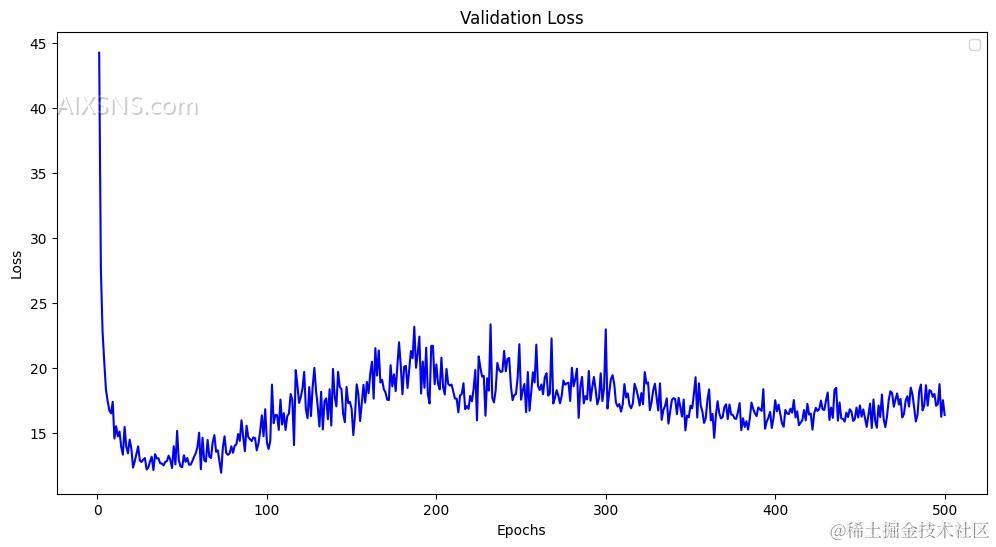
LOSS

In [14]:

num_epochs

Out[14]:

500

In [15]:

epochs = range(1, num_epochs+ 1)  # 作为横轴

plt.figure(figsize=(12,6))
plt.plot(epochs, loss_val_average, "blue")
plt.xlabel("Epochs")
plt.ylabel("Loss")

plt.legend()
plt.title("Validation Loss")
plt.show()

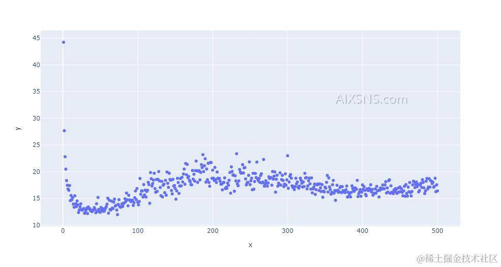
基于plotly绘制图像：

In [16]:

import plotly_express as px

px.scatter(x=epochs,y=loss_val_average)

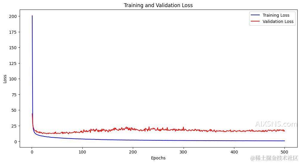
In [17]:

epochs = range(1, num_epochs+ 1)  # 作为横轴

plt.figure(figsize=(12,6))

plt.plot(epochs, loss_average, "blue", label="Training Loss")
plt.plot(epochs, loss_val_average, "red", label="Validation Loss")
plt.xlabel("Epochs")
plt.ylabel("Loss")

plt.legend()
plt.title("Training and Validation Loss")
plt.show()

MAE

In [18]:

epochs = range(1, num_epochs+1)  # 作为横轴

plt.plot(epochs, mae_average, "blue", label="Training MAE")
plt.plot(epochs, mae_val_average, "red", label="Validation MAE")
plt.xlabel("Epochs")
plt.ylabel("MAE")

plt.legend()
plt.title("Training and Validation MAE")
plt.show()

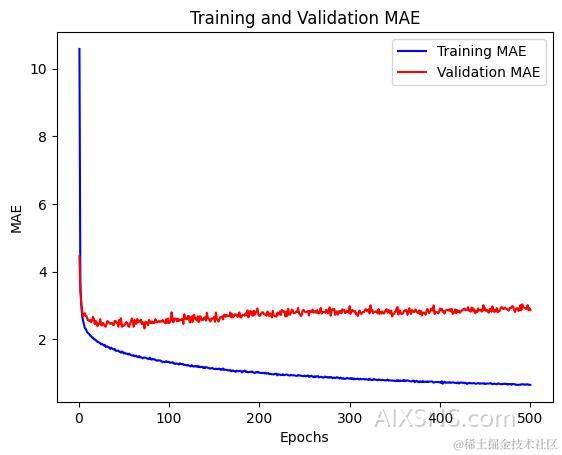
模型优化

可以看到，在训练集或者验证集上，不管是损失Loss还是误差MAE，前面的10个数据点和其他点差异很大，属于异常值，考虑直接删除。

数据的平滑处理：将每个数据点替换为前面数据点的平均值，得到较为光滑的曲线。

In [19]:

def smooth(points, factor=0.9):
    smooth_points = []

    for point in points:
        if smooth_points: 
            previous = smooth_points[-1]
            smooth_points.append(previous * factor + point * (1 - factor)) # 前一个点 * 0.9 + 当前点 * 0.1
        else:  # 不存在元素则添加point点
            smooth_points.append(point)
                
    return smooth_points

排除前10个点后进行平滑处理：

In [20]:

smooth_mae = smooth(mae_average[10:]) 
smooth_mae_val = smooth(mae_val_average[10:]) 
smooth_loss = smooth(loss_average[10:]) 
smooth_loss_val = smooth(loss_val_average[10:]) 

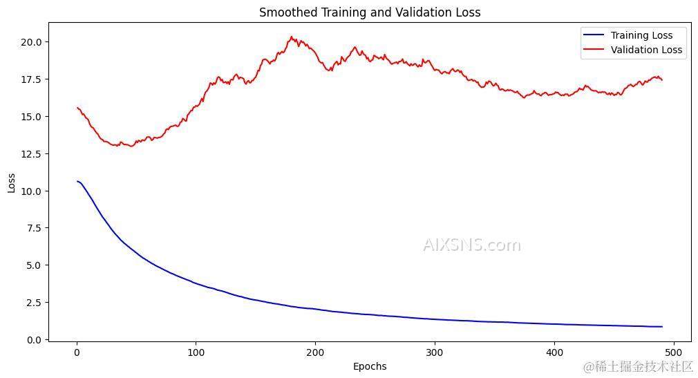
新LOSS

In [21]:

epochs = range(1, len(smooth_mae)+ 1)  # 作为横轴

plt.figure(figsize=(12,6))

plt.plot(epochs, smooth_loss, "blue", label="Training Loss")
plt.plot(epochs, smooth_loss_val, "red", label="Validation Loss")
plt.xlabel("Epochs")
plt.ylabel("Loss")

plt.legend()
plt.title("Smoothed Training and Validation Loss")
plt.show()

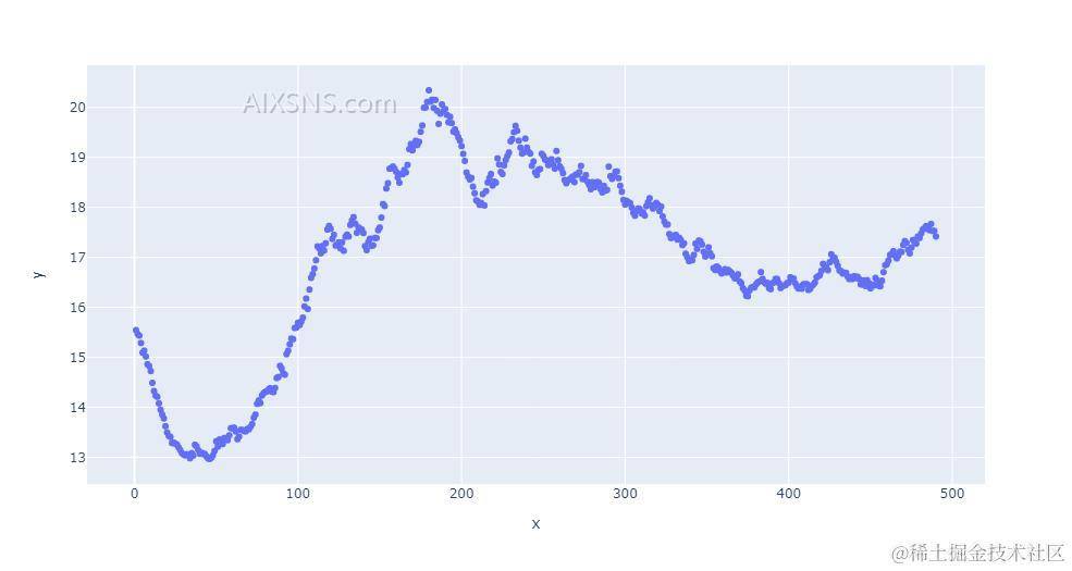
# fig = px.scatter(x=epochs, y=smooth_mae)
fig = px.scatter(x=epochs, y=smooth_loss_val)

fig.show()

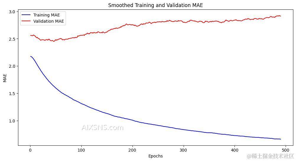
新MAE

In [23]:

epochs = range(1, len(smooth_mae)+ 1)  # 作为横轴

plt.figure(figsize=(12,6))

plt.plot(epochs, smooth_mae, "blue", label="Training MAE")
plt.plot(epochs, smooth_mae_val, "red", label="Validation MAE")
plt.xlabel("Epochs")
plt.ylabel("MAE")

plt.legend()
plt.title("Smoothed Training and Validation MAE")
plt.show()

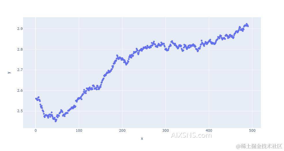
# fig = px.scatter(x=epochs, y=smooth_mae)
fig = px.scatter(x=epochs, y=smooth_mae_val) 

fig.show()

可以看到：在训练集上loss和mae随着轮次的进行，都在逐渐变小；但是在验证集上，并非如此，在50轮左右降到最低；