持续创作,加速成长!这是我参与「掘金日新计划 · 10 月更文挑战」的第25天,Failing Loudly: An Empirical Study of Methods for Detecting Dataset Shift 中的建议,我们将未经训练的自动编码器 (UAE) 和使用分类器的 softmax 输出 (BBSD) 的黑盒漂移检测作为开箱即用的预处理方法;同时, PCA 也可以使用 scikit-learn 轻松实现。
不依赖分类器的预处理方法通常会发现输入数据中的漂移,而 BBSD 则侧重于标签漂移。作为库的一部分的对抗性检测器也可以转换为漂移检测器,用于检测降低分类模型性能的漂移。
因此,我们可以结合不同的预处理技术来确定是否存在损害模型性能的漂移,以及这种漂移是否可以归类为输入漂移或标签漂移。
后端
该方法适用于 PyTorch 和 TensorFlow 框架,用于统计测试和预处理步骤。 但是 Alibi Detect 不会为您安装 PyTorch。 如何执行此操作请查看 Failing Loudly:An Empirical Study of Methods for Detecting Dataset Shift 中也使用了一些降维方法:随机初始化的编码器(论文中的 UAE 或未经训练的自动编码器)、BBSD(使用分类器的 softmax 输出的黑盒漂移检测) 和 PCA。
随机编码器
首先我们尝试随机初始化的编码器:
from functools import partial
from tensorflow.keras.layers import Conv2D, Dense, Flatten, InputLayer, Reshape
from alibi_detect.cd.tensorflow import preprocess_drift

tf.random.set_seed(0)

# define encoder
encoding_dim = 32
encoder_net = tf.keras.Sequential(
  [
      InputLayer(input_shape=(32, 32, 3)),
      Conv2D(64, 4, strides=2, padding='same', activation=tf.nn.relu),
      Conv2D(128, 4, strides=2, padding='same', activation=tf.nn.relu),
      Conv2D(512, 4, strides=2, padding='same', activation=tf.nn.relu),
      Flatten(),
      Dense(encoding_dim,)
  ]
)

# define preprocessing function
preprocess_fn = partial(preprocess_drift, model=encoder_net, batch_size=512)

# initialise drift detector
p_val = .05
cd = KSDrift(X_ref, p_val=p_val, preprocess_fn=preprocess_fn)


# we can also save/load an initialised detector
filepath = 'my_path'  # change to directory where detector is saved
save_detector(cd, filepath)
cd = load_detector(filepath)
运行结果:
WARNING:tensorflow:Compiled the loaded model, but the compiled metrics have yet to be built. `model.compile_metrics` will be empty until you train or evaluate the model.
WARNING:tensorflow:No training configuration found in the save file, so the model was *not* compiled. Compile it manually.
由于 Bonferroni 校正,检测器对具有 encoding_dim 特征的多元数据使用的 p 值等于 p_val / encoding_dim。
assert cd.p_val / cd.n_features == p_val / encoding_dim
让我们检查检测器是否认为漂移发生在不同的测试集和预测调用的时间:
from timeit import default_timer as timer

labels = ['No!', 'Yes!']

def make_predictions(cd, x_h0, x_corr, corruption):
    t = timer()
    preds = cd.predict(x_h0)
    dt = timer() - t
    print('No corruption')
    print('Drift? {}'.format(labels[preds['data']['is_drift']]))
    print('Feature-wise p-values:')
    print(preds['data']['p_val'])
    print(f'Time (s) {dt:.3f}')

    # 扰动数据
    if isinstance(x_corr, list):
        for x, c in zip(x_corr, corruption):
            t = timer()
            preds = cd.predict(x)
            dt = timer() - t
            print('')
            print(f'Corruption type: {c}')
            print('Drift? {}'.format(labels[preds['data']['is_drift']]))
            print('Feature-wise p-values:')
            print(preds['data']['p_val'])
            print(f'Time (s) {dt:.3f}')
make_predictions(cd, X_h0, X_c, corruption)
运行结果:
No corruption
Drift? No!
Feature-wise p-values:
[0.9386024  0.13979132 0.6384489  0.05413922 0.37460664 0.25598603 0.87304014 0.47553554 0.11587767 0.67217577 0.47553554 0.7388285 0.08215971 0.14635575 0.3114053  0.3114053  0.60482025 0.36134896 0.8023182  0.21715216 0.24582714 0.46030036 0.11587767 0.44532147 0.25598603 0.58811766 0.5550683  0.95480835 0.8598946  0.23597081 0.8975547  0.68899393]
Time (s) 1.172

Corruption type: gaussian_noise
Drift? Yes!
Feature-wise p-values:
[4.85834153e-03 7.20506581e-03 5.44517934e-02 9.87569049e-09 3.35018486e-01 8.05620551e-02 6.66609779e-03 2.68237293e-01 1.52247362e-02 1.01558706e-02 1.78680534e-03 1.04267694e-01 4.93385670e-08 1.35106135e-10 1.04696119e-04 1.35730659e-06 2.87180692e-01 3.79266362e-06 3.45018925e-04 1.96636513e-01 1.86571106e-03 5.92635339e-03 4.70917694e-10 5.92635339e-03 5.07743537e-01 5.31427140e-05 3.80059540e-01 1.13354892e-01 2.75738519e-02 7.75579622e-07 3.23252240e-03 2.02312917e-02]
Time (s) 2.516

Corruption type: motion_blur
Drift? Yes!
Feature-wise p-values:
[3.39037769e-07 1.16525307e-01 5.04726835e-04 3.81079665e-03 6.31192625e-01 5.28989534e-04 3.61990853e-04 1.57829020e-02 1.94784126e-03 1.26909809e-02 4.46249526e-09 6.99155149e-04 3.79746925e-04 5.88651128e-21 1.35596551e-07 2.00218983e-05 7.15865940e-02 7.28750820e-05 1.04267694e-01 1.10198918e-04 2.22608112e-04 1.52403876e-01 6.41064299e-03 3.15323919e-02 3.04985344e-02 8.97102946e-05 6.54255822e-02 2.03331537e-03 1.15137536e-03 8.04463718e-10 9.62164486e-04 3.45018925e-04]
Time (s) 2.622

Corruption type: brightness
Drift? Yes!
Feature-wise p-values:
[0.0000000e+00 0.0000000e+00 4.0479114e-29 0.0000000e+00 0.0000000e+00 0.0000000e+00 0.0000000e+00 0.0000000e+00 0.0000000e+00 0.0000000e+00 0.0000000e+00 0.0000000e+00 0.0000000e+00 2.3823024e-21 2.9582986e-38 0.0000000e+00 0.0000000e+00 0.0000000e+00 7.1651735e-34 0.0000000e+00 0.0000000e+00 0.0000000e+00 0.0000000e+00 0.0000000e+00 0.0000000e+00 3.8567345e-05 0.0000000e+00 0.0000000e+00 0.0000000e+00 0.0000000e+00 0.0000000e+00 0.0000000e+00]
Time (s) 2.572

Corruption type: pixelate
Drift? Yes!
Feature-wise p-values:
[3.35018486e-01 2.06576437e-01 1.96636513e-01 8.40378553e-03 5.92454255e-01 9.30991620e-02 1.64748102e-01 5.16919196e-01 2.40608733e-02 4.54285979e-01 1.91894709e-04 1.33487985e-01 1.63820793e-03 1.78680534e-03 1.13354892e-01 9.04688612e-02 8.27570856e-01 6.15745559e-02 6.54255822e-02 9.06871445e-03 2.38713458e-01 6.89552963e-01 1.07227206e-01 8.29487666e-02 3.42268527e-01 1.37110472e-01 3.64637136e-01 3.00327957e-01 3.72297794e-01 9.06871445e-03 4.98639137e-01 9.78103094e-03]
Time (s) 2.554
正如预期的那样,仅在损坏的数据集上检测到漂移。
在多变量校正之前,每个(编码)特征的每个单变量 K-S 检验的特征 p 值表明,对于 H0 数据集它们中的大多数远高于阈值(0.05),而对于损坏的数据集则低于此阈值。
BBSD
对于 BBSD,我们使用分类器的 softmax 输出进行黑盒漂移检测。 此方法基于使用黑盒预测器检测和校正标签漂移。 ResNet 分类器是根据实例标准化的数据进行训练的,因此我们需要重新调整数据。
X_train = scale_by_instance(X_train)
X_test = scale_by_instance(X_test)

X_ref = scale_by_instance(X_ref)
X_h0 = scale_by_instance(X_h0)

X_c = [scale_by_instance(X_c[i]) for i in range(n_corr)]
现在我们初始化检测器。 这里我们使用 softmax 层的输出来检测漂移,但也可以通过将“layer”设置为模型中所需隐藏层的索引来提取其他隐藏层:
from alibi_detect.cd.tensorflow import HiddenOutput

# define preprocessing function, we use the
preprocess_fn = partial(preprocess_drift, model=HiddenOutput(clf, layer=-1), batch_size=128)

cd = KSDrift(X_ref, p_val=p_val, preprocess_fn=preprocess_fn)
我们再次可以看到,由于 Bonferroni 校正,检测器对具有 10 个特征(CIFAR-10 类的数量)的多元数据使用的 p 值等于 p_val / 10。
assert cd.p_val / cd.n_features == p_val / 10
原始测试集没有漂移:
make_predictions(cd, X_h0, X_c, corruption)
No corruption
Drift? No!
Feature-wise p-values:
[0.11587767 0.5226477  0.19109942 0.19949944 0.49101472 0.722359 0.12151605 0.41617486 0.8320209  0.75510186]
Time (s) 7.608

Corruption type: gaussian_noise
Drift? Yes!
Feature-wise p-values:
[0. 0. 0. 0. 0. 0. 0. 0. 0. 0.]
Time (s) 16.233

Corruption type: motion_blur
Drift? Yes!
Feature-wise p-values:
[0. 0. 0. 0. 0. 0. 0. 0. 0. 0.]
Time (s) 15.688

Corruption type: brightness
Drift? Yes!
Feature-wise p-values:
[0.0000000e+00 3.8790170e-15 2.2549014e-33 4.6733894e-07 2.1857751e-15 1.2091652e-05 2.3977423e-30 1.0099583e-09 4.3286997e-12 3.8117909e-17]
Time (s) 14.733

Corruption type: pixelate
Drift? Yes!
Feature-wise p-values:
[0. 0. 0. 0. 0. 0. 0. 0. 0. 0.]
Time (s) 13.781
标签漂移
我们还可以检查当我们在参考数据 X_ref 和测试数据 X_imb 之间引入类不平衡时会发生什么。 参考数据将使用前 5 个类的 75% 的实例,而仅使用后 5 个类的 25%。然后,用于漂移测试的数据分别使用前 5 个类和后 5 个类的 25% 和 75% 的测试实例。
np.random.seed(0)

# get index for each class in the test set
num_classes = len(np.unique(y_test))
# 在测试数据集中获取每个类的索引
idx_by_class = [np.where(y_test == c)[0] for c in range(num_classes)]

# sample imbalanced data for different classes for X_ref and X_imb
perc_ref = .75
# 计算每个类的百分比,前五个类:0.75,后五个类:0.25
perc_ref_by_class = [perc_ref if c < 5 else 1 - perc_ref for c in range(num_classes)]

# 每个类的数量
n_by_class = n_test // num_classes

X_ref = []
X_imb, y_imb = [], []
for _ in range(num_classes):
    # 获取每个类的采样索引
    idx_class_ref = np.random.choice(n_by_class, size=int(perc_ref_by_class[_] * n_by_class), replace=False)
    # 获取每个类的采样值
    idx_ref = idx_by_class[_][idx_class_ref]

    idx_class_imb = np.delete(np.arange(n_by_class), idx_class_ref, axis=0)
    idx_imb = idx_by_class[_][idx_class_imb]

    assert not np.array_equal(idx_ref, idx_imb)

    X_ref.append(X_test[idx_ref])
    X_imb.append(X_test[idx_imb])
    y_imb.append(y_test[idx_imb])

# 将每个类合并到一起
X_ref = np.concatenate(X_ref)
X_imb = np.concatenate(X_imb)
y_imb = np.concatenate(y_imb)

print(X_ref.shape, X_imb.shape, y_imb.shape)
运行结果:
(5000, 32, 32, 3) (5000, 32, 32, 3) (5000,)
更新检测器的参考数据集并进行预测。
注意:
我们存储预处理的参考数据;因为,kwarg参数
preprocess_at_init默认为 True:
cd.x_ref = cd.preprocess_fn(X_ref)
preds_imb = cd.predict(X_imb)
print('Drift? {}'.format(labels[preds_imb['data']['is_drift']]))
print(preds_imb['data']['p_val'])
运行结果:
Drift? Yes!
[5.2598997e-20 1.1312397e-20 5.8646589e-29 9.2977640e-18 6.4071548e-23
 1.4155961e-15 5.0236095e-19 1.6651963e-20 4.2726706e-21 3.5123729e-21]
更新参考数据
到目前为止,我们在整个实验中保持参考数据相同。 然而,我们可能希望针对最后 N 个实例或针对一批固定大小的实例测试一个新批次,其中我们为到目前为止我们看到的每个实例提供相同的机会进入参考批次(蓄水池采样)。
update_x_ref 参数允许您更改参考数据更新规则。 它是一个字典,它将更新规则(最后 N 个实例的’last’或’reservoir_sampling’)作为键,并将参考数据的批大小 N 作为值。
您还可以在预测调用后保存检测器以保存更新的参考数据。
N = 7500
cd = KSDrift(X_ref, p_val=.05, preprocess_fn=preprocess_fn, update_x_ref={'reservoir_sampling': N})
现在,每次predict调用都会更新参考数据。 假设我们从不平衡的参考集开始,对剩余的测试集数据 X_imb 进行预测;然后,漂移检测器会发现数据漂移已经发生。
preds_imb = cd.predict(X_imb)
print('Drift? {}'.format(labels[preds_imb['data']['is_drift']]))
运行结果:
Drift? Yes!
我们现在可以看到参考数据由 N 个实例组成,这些实例是通过蓄水池(reservoir)采样获得的。
assert cd.x_ref.shape[0] == N
然后,我们从训练集中抽取一个随机样本,并将其与更新的参考数据进行比较。这仍然突出显示存在数据漂移,但将再次更新参考数据:
np.random.seed(0)

perc_train = .5
n_train = X_train.shape[0]

idx_train = np.random.choice(n_train, size=int(perc_train * n_train), replace=False)
preds_train = cd.predict(X_train[idx_train])
print('Drift? {}'.format(labels[preds_train['data']['is_drift']]))
运行结果:
Drift? Yes!
当我们从训练集中提取新样本时,它突出显示出它不再在 X_ref 中的蓄水池(reservoir)上漂移。
np.random.seed(1)

perc_train = .1
idx_train = np.random.choice(n_train, size=int(perc_train * n_train), replace=False)

preds_train = cd.predict(X_train[idx_train])
print('Drift? {}'.format(labels[preds_train['data']['is_drift']]))
运行结果:
Drift? No!
多元校正机制
除了多变量数据的 Bonferroni 校正,我们还可以使用不太保守的错误发现率 (FDR) 校正。 请参阅此处或此处以获得很好的解释。 Bonferroni 校正控制了至少一个误报的概率,而 FDR 校正控制了预期的误报数量。 当应用 FDR 校正时,初始化时的 p_val 参数可以解释为可接受的 q 值。
cd = KSDrift(X_ref, p_val=.05, preprocess_fn=preprocess_fn, correction='fdr')

preds_imb = cd.predict(X_imb)
print('Drift? {}'.format(labels[preds_imb['data']['is_drift']]))
运行结果:
Drift? Yes!
将对抗性自动编码器作为恶意漂移检测器
我们可以利用从对正常数据进行训练的对抗性自动编码器获得的对抗性分数,并将其转换为数据漂移检测器。 对抗性自动编码器的得分函数成为漂移检测器的预处理函数。
K-S 检验是对抗性分数的简单单变量测试。 重要的是,对抗性漂移检测器会标记恶意数据漂移。 我们可以从 Google Cloud Bucket 中获取预训练的对抗检测器,或者从头开始训练:
load_pretrained = True
from tensorflow.keras.regularizers import l1
from tensorflow.keras.layers import Conv2DTranspose
from alibi_detect.ad import AdversarialAE

# change filepath to (absolute) directory where model is downloaded
filepath = os.path.join(os.getcwd(), 'my_path')
detector_type = 'adversarial'
detector_name = 'base'
filepath = os.path.join(filepath, detector_name)

if load_pretrained:
    ad = fetch_detector(filepath, detector_type, dataset, detector_name, model=model)
else:  # train detector from scratch 从头开始训练检测器
    # 定义编码和解码网络
    # define encoder and decoder networks
    encoder_net = tf.keras.Sequential(
            [
                InputLayer(input_shape=(32, 32, 3)),
                Conv2D(32, 4, strides=2, padding='same',
                       activation=tf.nn.relu, kernel_regularizer=l1(1e-5)),
                Conv2D(64, 4, strides=2, padding='same',
                       activation=tf.nn.relu, kernel_regularizer=l1(1e-5)),
                Conv2D(256, 4, strides=2, padding='same',
                       activation=tf.nn.relu, kernel_regularizer=l1(1e-5)),
                Flatten(),
                Dense(40)
            ]
        )

    decoder_net = tf.keras.Sequential(
        [
                InputLayer(input_shape=(40,)),
                Dense(4 * 4 * 128, activation=tf.nn.relu),
                Reshape(target_shape=(4, 4, 128)),
                Conv2DTranspose(256, 4, strides=2, padding='same',
                                activation=tf.nn.relu, kernel_regularizer=l1(1e-5)),
                Conv2DTranspose(64, 4, strides=2, padding='same',
                                activation=tf.nn.relu, kernel_regularizer=l1(1e-5)),
                Conv2DTranspose(3, 4, strides=2, padding='same',
                                activation=None, kernel_regularizer=l1(1e-5))
            ]
        )

    # 初始化和训练检测器
    # initialise and train detector
    ad = AdversarialAE(encoder_net=encoder_net, decoder_net=decoder_net, model=clf)
    ad.fit(X_train, epochs=50, batch_size=128, verbose=True)

    # 保存训练对抗性检测器
    # save the trained adversarial detector
    save_detector(ad, filepath)
初始化漂移检测器:
np.random.seed(0)
idx = np.random.choice(n_test, size=n_test // 2, replace=False)
X_ref = scale_by_instance(X_test[idx])

# 对抗性分数
# adversarial score fn = preprocess step
preprocess_fn = partial(ad.score, batch_size=128)

cd = KSDrift(X_ref, p_val=.05, preprocess_fn=preprocess_fn)
对原始测试集和损坏的数据进行漂移预测:
clf_accuracy['h0'] = clf.evaluate(X_h0, y_h0, batch_size=128, verbose=0)[1]
preds_h0 = cd.predict(X_h0)
print('H0: Accuracy {:.4f} -- Drift? {}'.format(
    clf_accuracy['h0'], labels[preds_h0['data']['is_drift']]))

clf_accuracy['imb'] = clf.evaluate(X_imb, y_imb, batch_size=128, verbose=0)[1]
preds_imb = cd.predict(X_imb)
print('imbalance: Accuracy {:.4f} -- Drift? {}'.format(
    clf_accuracy['imb'], labels[preds_imb['data']['is_drift']]))

for x, c in zip(X_c, corruption):
    preds = cd.predict(x)
    print('{}: Accuracy {:.4f} -- Drift? {}'.format(
        c, clf_accuracy[c],labels[preds['data']['is_drift']]))
运行结果:
H0: Accuracy 0.9286 -- Drift? No!
imbalance: Accuracy 0.9282 -- Drift? No!

gaussian_noise: Accuracy 0.2208 -- Drift? Yes!
motion_blur: Accuracy 0.6339 -- Drift? Yes!
brightness: Accuracy 0.8913 -- Drift? Yes!
pixelate: Accuracy 0.3666 -- Drift? Yes!
虽然 X_imb 由于引入的类不平衡而明显表现出输入数据漂移,但它不会被对抗性漂移检测器标记,因为分类器的性能不受影响并且漂移不是恶意的。
我们可以通过将对抗分数与分类器准确性下降所反映的数据损坏的危害性一起绘制来可视化这一点:
adv_scores = {}

score = ad.score(X_ref, batch_size=128)
adv_scores['original'] = {'mean': score.mean(), 'std': score.std()}

score = ad.score(X_h0, batch_size=128)
adv_scores['h0'] = {'mean': score.mean(), 'std': score.std()}

score = ad.score(X_imb, batch_size=128)
adv_scores['imb'] = {'mean': score.mean(), 'std': score.std()}

for x, c in zip(X_c, corruption):
    score_x = ad.score(x, batch_size=128)
    adv_scores[c] = {'mean': score_x.mean(), 'std': score_x.std()}
mu = [v['mean'] for _, v in adv_scores.items()]
stdev = [v['std'] for _, v in adv_scores.items()]
xlabels = list(adv_scores.keys())
acc = [clf_accuracy[label] for label in xlabels]
xticks = np.arange(len(mu))

width = .35

fig, ax = plt.subplots()
ax2 = ax.twinx()

p1 = ax.bar(xticks, mu, width, yerr=stdev, capsize=2)
color = 'tab:red'
p2 = ax2.bar(xticks + width, acc, width, color=color)

ax.set_title('Adversarial Scores and Accuracy by Corruption Type')
ax.set_xticks(xticks + width / 2)
ax.set_xticklabels(xlabels, rotation=45)
ax.legend((p1[0], p2[0]), ('Score', 'Accuracy'), loc='upper right', ncol=2)
ax.set_ylabel('Adversarial Score')

color = 'tab:red'
ax2.set_ylabel('Accuracy')
ax2.set_ylim((-.26,1.2))
ax.set_ylim((-2,9))

plt.show()
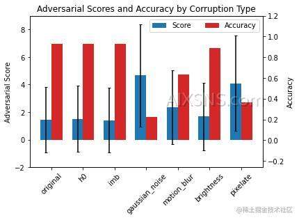
因此,我们可以使用检测器本身的分数来量化漂移的危害! 我们可以将其推广到 CIFAR-10-C 中每个严重级别的所有损坏:
def accuracy(y_true: np.ndarray, y_pred: np.ndarray) -> float:
    return (y_true == y_pred).astype(int).sum() / y_true.shape[0]
from alibi_detect.utils.tensorflow import predict_batch

severities = [1, 2, 3, 4, 5]

score_drift = {
    1: {'all': [], 'harm': [], 'noharm': [], 'acc': 0},
    2: {'all': [], 'harm': [], 'noharm': [], 'acc': 0},
    3: {'all': [], 'harm': [], 'noharm': [], 'acc': 0},
    4: {'all': [], 'harm': [], 'noharm': [], 'acc': 0},
    5: {'all': [], 'harm': [], 'noharm': [], 'acc': 0},
}

y_pred = predict_batch(X_test, clf, batch_size=256).argmax(axis=1)

score_x = ad.score(X_test, batch_size=256)

for s in severities:
    print('nSeverity: {} of {}'.format(s, len(severities)))

    print('Loading corrupted dataset...')
    X_corr, y_corr = fetch_cifar10c(corruption=corruptions, severity=s, return_X_y=True)
    X_corr = X_corr.astype('float32')

    # 预处理
    print('Preprocess data...')
    X_corr = scale_by_instance(X_corr)

    print('Make predictions on corrupted dataset...')
    y_pred_corr = predict_batch(X_corr, clf, batch_size=256).argmax(axis=1)

    # 在损坏数据集计算对抗分数
    print('Compute adversarial scores on corrupted dataset...')
    score_corr = ad.score(X_corr, batch_size=256)

    print('Get labels for malicious corruptions...')
    labels_corr = np.zeros(score_corr.shape[0])
    repeat = y_corr.shape[0] // y_test.shape[0]
    y_pred_repeat = np.tile(y_pred, (repeat,))
    # malicious/harmful corruption: original prediction correct but
    # prediction on corrupted data incorrect
    idx_orig_right = np.where(y_pred_repeat == y_corr)[0]
    idx_corr_wrong = np.where(y_pred_corr != y_corr)[0]
    idx_harmful = np.intersect1d(idx_orig_right, idx_corr_wrong)
    labels_corr[idx_harmful] = 1
    labels = np.concatenate([np.zeros(X_test.shape[0]), labels_corr]).astype(int)
    # harmless corruption: original prediction correct and prediction
    # on corrupted data correct
    idx_corr_right = np.where(y_pred_corr == y_corr)[0]
    idx_harmless = np.intersect1d(idx_orig_right, idx_corr_right)

    score_drift[s]['all'] = score_corr
    score_drift[s]['harm'] = score_corr[idx_harmful]
    score_drift[s]['noharm'] = score_corr[idx_harmless]
    score_drift[s]['acc'] = accuracy(y_corr, y_pred_corr)
运行结果:
Severity: 1 of 5
Loading corrupted dataset...
Preprocess data...
Make predictions on corrupted dataset...
Compute adversarial scores on corrupted dataset...
Get labels for malicious corruptions...

Severity: 2 of 5
Loading corrupted dataset...
Preprocess data...
Make predictions on corrupted dataset...
Compute adversarial scores on corrupted dataset...
Get labels for malicious corruptions...

Severity: 3 of 5
Loading corrupted dataset...
Preprocess data...
Make predictions on corrupted dataset...
Compute adversarial scores on corrupted dataset...
Get labels for malicious corruptions...

Severity: 4 of 5
Loading corrupted dataset...
Preprocess data...
Make predictions on corrupted dataset...
Compute adversarial scores on corrupted dataset...
Get labels for malicious corruptions...

Severity: 5 of 5
Loading corrupted dataset...
Preprocess data...
Make predictions on corrupted dataset...
Compute adversarial scores on corrupted dataset...
Get labels for malicious corruptions...
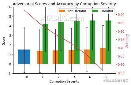
我们现在计算每个严重级别的平均分数和标准偏差并绘制结果。
该图显示了提高数据损坏严重程度的平均对抗分数 (lhs) 和 ResNet-32 准确度 (rhs)。 级别 0 对应于原始测试集。有害分数是由于损坏而从正确预测变为错误预测的实例的分数。无害意味着预测在损坏后没有改变。
mu_noharm, std_noharm = [], []
mu_harm, std_harm = [], []
acc = [clf_accuracy['original']]

for k, v in score_drift.items():
    # 无害
    mu_noharm.append(v['noharm'].mean())
    std_noharm.append(v['noharm'].std())
    # 有害
    mu_harm.append(v['harm'].mean())
    std_harm.append(v['harm'].std())
    acc.append(v['acc'])
plot_labels = ['0', '1', '2', '3', '4', '5']

N = 6
ind = np.arange(N)
width = .35

fig_bar_cd, ax = plt.subplots()
ax2 = ax.twinx()

p0 = ax.bar(ind[0], score_x.mean(), yerr=score_x.std(), capsize=2)
p1 = ax.bar(ind[1:], mu_noharm, width, yerr=std_noharm, capsize=2)
p2 = ax.bar(ind[1:] + width, mu_harm, width, yerr=std_harm, capsize=2)

ax.set_title('Adversarial Scores and Accuracy by Corruption Severity')
ax.set_xticks(ind + width / 2)
ax.set_xticklabels(plot_labels)
ax.set_ylim((-1,6))
ax.legend((p1[0], p2[0]), ('Not Harmful', 'Harmful'), loc='upper right', ncol=2)
ax.set_ylabel('Score')
ax.set_xlabel('Corruption Severity')

color = 'tab:red'
ax2.set_ylabel('Accuracy', color=color)
ax2.plot(acc, color=color)
ax2.tick_params(axis='y', labelcolor=color)

plt.show()
原文链接:Kolmogorov-Smirnov data drift detector on CIFAR-10
