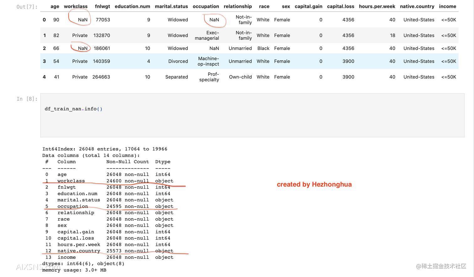
本次课程依旧使用人口普查数据, 上次课中，当我们对类别型变量编码的时候，就发现某些列中有？（问号），这是因为此数据集中，当某人在做问卷调查未回答某个问题时，该空缺用？填充（不同数据集用不同符号表示缺失）

因此我们需要面对如何处理缺失值（missing values）的问题，最简单粗暴的办法是某一行如果包含缺失值就丢掉，但此种方法最大的问题是： 如果模型部署后，新来的数据中有缺失值呢？ 或者缺失值很多呢，都删掉就会丢掉很多本可以用的数据

所以有必要掌握sklearn中一些处理缺失值的办法，关于该主题如果想深入了解，需去统计学课程中寻找答案

缺失值处理 （简易版）

import pandas as pd
import numpy as np
import matplotlib.pyplot as plt
plt.rcParams['font.size'] = 16

from sklearn.dummy import DummyClassifier
from sklearn.tree import DecisionTreeClassifier
from sklearn.linear_model import LogisticRegression
from sklearn.model_selection import train_test_split, cross_val_score, cross_validate, GridSearchCV, RandomizedSearchCV
from sklearn.preprocessing import OneHotEncoder, OrdinalEncoder
from sklearn.pipeline import Pipeline
from sklearn.preprocessing import StandardScaler, MinMaxScaler
from sklearn.compose import ColumnTransformer
from sklearn import set_config, config_context

census = pd.read_csv('data/adult.csv')
# 上节课提到过可以删除 `education` 列，
# 因为数据集中已经有一列顺序编码过的列 `education.num`.
census = census.drop(columns=["education"])

census_train, census_test = train_test_split(census, test_size=0.2, random_state=123)

# 把代表缺失值的问号，替换为Pandas中标准的 np.NaN
# 这里好像有破坏了 golden rule的嫌疑，对test set进行了操作
# 但我们可以这样理解： 假如原始csv格式的数据中，对缺失值的表示就是标准的，就不需要这一步了，所以说，这里并不算破坏了 golden rule
# 个人理解这一步甚至可以提前到 train_test_split之前，只是为了让同学们养成好习惯，这里放在了之后
df_train_nan = census_train.replace('?', np.NaN)
df_test_nan  = census_test.replace( '?', np.NaN)

df_train_nan.sort_index().head()

注意：这里我们处理的是特征列中的缺失值，而不是目标列income中的缺失值，
因为我们做的是监督学习，如果income中有缺失值，那这一行可以考虑删掉

X_train_nan = df_train_nan.drop(columns=['income'])
X_test_nan  = df_test_nan.drop(columns=['income'])
y_train = df_train_nan['income']
y_test = df_test_nan['income']

Imputation 插值

• Imputation means inventing values for the missing data.
• The strategies are different for numeric(mean, median…) vs. categorical.
• In this dataset it turns out we only have missing values in the categorical features.

from sklearn.impute import SimpleImputer

imp = SimpleImputer(strategy='most_frequent')

• This imputer is another transformer, like the other ones we’ve seen (CountVectorizer, OrdinalEncoder, OneHotEncoder).

numeric_features = ['age', 'fnlwgt', 'education.num', 'capital.gain', 
                    'capital.loss', 'hours.per.week']
categorical_features = ['workclass', 'marital.status', 'occupation', 
                        'relationship', 'race', 'sex', 'native.country']
target_column = 'income'


imp.fit(X_train_nan[categorical_features]);

X_train_imp_cat = pd.DataFrame(imp.transform(X_train_nan[categorical_features]),
                           columns=categorical_features, index=X_train_nan.index)
X_test_imp_cat = pd.DataFrame(imp.transform(X_test_nan[categorical_features]),
                           columns=categorical_features, index=X_test_nan.index)

X_train_imp = X_train_nan.copy()
X_train_imp.update(X_train_imp_cat)

X_test_imp = X_test_nan.copy()
X_test_imp.update(X_test_imp_cat)

# 至此，所有的缺失值被 most_frequent 策略填充

另一种方法是，人为指定一个固定值插入:

# or just leave in the "?" and have this be its own category for categorical variables.
SimpleImputer(strategy='constant', fill_value="?");

Pipeline

至此，我们可以建立一个3阶段的Pipeline, 先回顾一下Pipeline的执行流程：

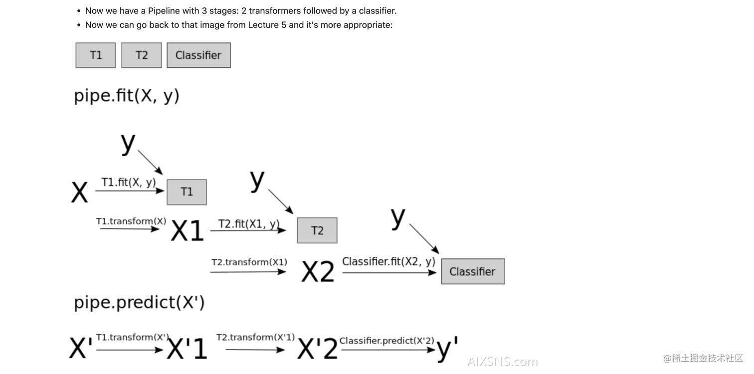
pipe = Pipeline([('imputation', SimpleImputer(strategy='most_frequent')),
                 ('ohe', OneHotEncoder(handle_unknown='ignore')),
                 ('lr', LogisticRegression(max_iter=1000))])
                 
pd.DataFrame(cross_validate(pipe, X_train_nan[categorical_features], y_train))
               

Feature scaling

不同于插值，特征缩放只适用于数值特征

为何要特征缩放

此处以逻辑回归为例，只用数据集中的数值型列来训练模型:

lr = LogisticRegression(max_iter=1000)
pd.DataFrame(cross_validate(lr, X_train_imp[numeric_features], y_train, return_train_score=True))

lr.fit(X_train_imp[numeric_features], y_train);

pd.DataFrame(data=lr.coef_[0], index=numeric_features, columns=['Coefficient'])

可以发现 fnlwgt （final weight）的系数非常小

提问：fnlwgt为何很小呢？我们来一起探究其原因：

X_train_nan.describe()

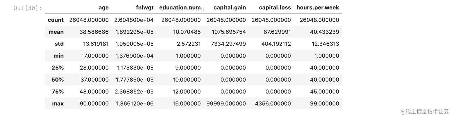
由统计结果可知，与其他几个数值型列相比，fnlwgt的平均值大约是200,000。我们来回忆逻辑回归，最终会给每个特征训练一个系数，推导时一条数据的每个特征乘以对应的系数，然后相加求和，最后使用sigmoid函数转换到0-1区间，所以说 fnlwgt本身很大，对应的系数就倾向于很小, 否则这一项就将主导整个预测。

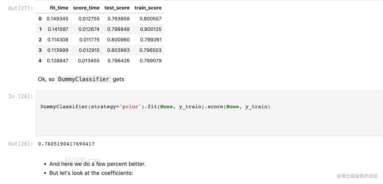
这有什么影响吗？我们来做个实验，把 fnlwgt 的单位修改，使每个数字都更大，同样办法把capital.gain、capital.loss的单位从dollars修改为 thousands of dollars，使数值变小，随后再训练逻辑回归，看看效果：

X_train_mod = X_train_imp[numeric_features].copy()
X_train_mod["capital.gain"] /= 1000
X_train_mod["capital.loss"] /= 1000
X_train_mod["fnlwgt"] *= 1000

X_train_mod.head()

lr = LogisticRegression(max_iter=1000)
pd.DataFrame(cross_validate(lr, X_train_mod, y_train, return_train_score=True)).mean()

# 输出:

fit_time       0.061292
score_time     0.012938
test_score     0.760519
train_score    0.760519
dtype: float64

此时会发现，整个模型的效果下降，连DummyClassifier都不如, 换句话说，此时的逻辑回归啥作用都没起，连瞎猜都不如。这一现象会在课程 CPSC340中得到解答，其实这里如果把逻辑回归的超参数C调大，也会减轻这一现象。

顺便一提，决策树就没有这个问题，因为它只考虑阈值，而不处理实际数字：

dt = DecisionTreeClassifier(random_state=1)
cross_val_score(dt, X_train_imp[numeric_features], y_train).mean() 
# 得分： 0.7707694308794502

# 在修改过单位的数据上使用
dt = DecisionTreeClassifier(random_state=1)
cross_val_score(dt, X_train_mod, y_train).mean()
# 得分一样： 0.7707694308794502

人们发现，这个问题会影响机器学习中的不少模型（原因需通过CPSC340学习了原理之后），所以还是养成好习惯（几乎没有任何伤害），专门处理一下该问题比较好，常见的方法就是对特征值缩放，下面我们具体讲两种缩放方法:

这一节我们只讲具体用法，而不关心他们各自的优缺点。

特征缩放之 Standardization

from sklearn.preprocessing import StandardScaler, MinMaxScaler

scaler = StandardScaler()
scaler.fit(X_train_imp[numeric_features]);

scaler.transform(X_train_imp[numeric_features])


scaled_train_df = pd.DataFrame(scaler.transform(X_train_imp[numeric_features]),
                           columns=numeric_features, index=X_train_imp.index)
                           
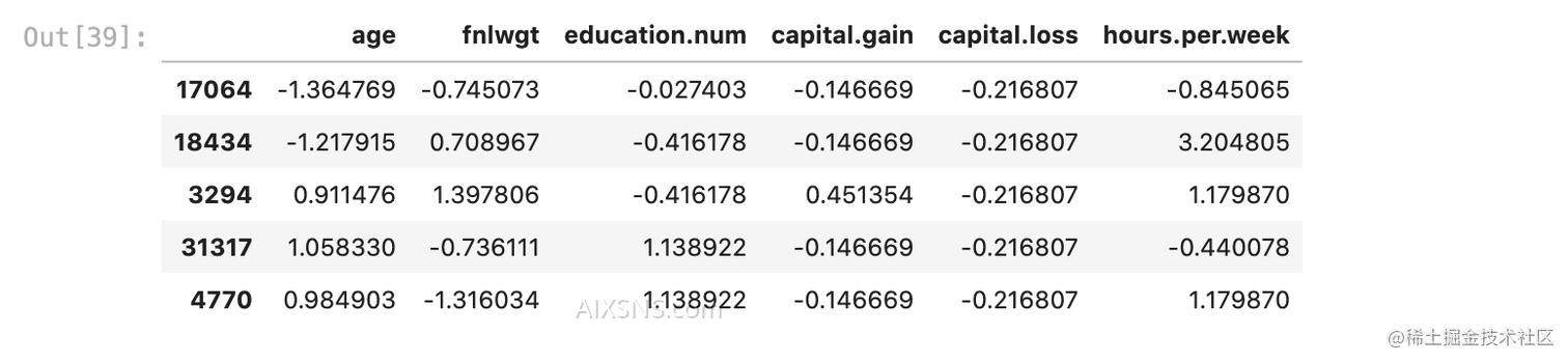
# 经过 standardization 之后                         
scaled_train_df.head()

# Let's check that it did what we expected:
scaled_train_df.mean(axis=0)

# 输出：
# These are basically all zero (10−16 is zero to numerical precision)
age               3.634832e-16
fnlwgt           -4.961863e-17
education.num     1.371028e-15
capital.gain     -3.863724e-16
capital.loss      7.671122e-16
hours.per.week    9.381657e-16
dtype: float64


scaled_train_df.std(axis=0)
# 输出:
age               1.000019
fnlwgt            1.000019
education.num     1.000019
capital.gain      1.000019
capital.loss      1.000019
hours.per.week    1.000019
dtype: float64

让我们继续上一节的实验，看看经过了standardization之后，模型效果是否提高, 先在原始数据查看：

# 1.  未修改的数据 Without scaling
lr = LogisticRegression(max_iter=1000)
pd.DataFrame(cross_validate(lr, X_train_imp[numeric_features], y_train, return_train_score=True)).mean()

# 结果:
fit_time       0.125385
score_time     0.012492
test_score     0.799217
train_score    0.799505
dtype: float64




# 2. 未修改的数据 With scaling
pipe = Pipeline([('scaling', StandardScaler()),
                 ('lr', LogisticRegression(max_iter=1000))])
pd.DataFrame(cross_validate(pipe, X_train_imp[numeric_features], y_train, return_train_score=True)).mean()

# 结果：
fit_time       0.061689
score_time     0.012663
test_score     0.814727
train_score    0.815024
dtype: float64

# 看得出，缩放之后确实有效果

再在修改过单位的数据上查看：

# 3. 修改过单位的数据 Without scaling
lr = LogisticRegression(max_iter=1000)
pd.DataFrame(cross_validate(lr, X_train_mod[numeric_features], y_train, return_train_score=True)).mean()

# 结果：
fit_time       0.061530
score_time     0.012299
test_score     0.760519
train_score    0.760519
dtype: float64


# 4. 修改过单位的数据 With scaling
pipe = Pipeline([('scaling', StandardScaler()),
                 ('lr', LogisticRegression(max_iter=1000))])
pd.DataFrame(cross_validate(pipe, X_train_mod[numeric_features], y_train, return_train_score=True)).mean()

# 结果：
fit_time       0.067296
score_time     0.013045
test_score     0.814727
train_score    0.815024
dtype: float64

# 缩放使得方差为1，所以我们修改数据时 乘以/除以1000的影响没有了

特征缩放之 Normalization

将刚才的对比换成 Normalization 缩放，很简单，只需将Pipeline中的 scaling组件替换:

# 未修改的数据 使用Normalization
pipe = Pipeline([('scaling', MinMaxScaler()),
                 ('lr', LogisticRegression(max_iter=1000))])
                 
pd.DataFrame(cross_validate(pipe, X_train_imp[numeric_features], y_train, return_train_score=True)).mean()

# 结果：
fit_time       0.086178
score_time     0.012658
test_score     0.810427
train_score    0.810888
dtype: float64

具体看一下 MinMaxScaler 做了什么：

minmax = MinMaxScaler()
minmax.fit(X_train_imp[numeric_features])
normalized_train = minmax.transform(X_train_imp[numeric_features])
normalized_test = minmax.transform(X_test_imp[numeric_features])

normalized_train.min(axis=0)
# 结果：
array([0., 0., 0., 0., 0., 0.])


normalized_train.max(axis=0)
# 结果:
array([1., 1., 1., 1., 1., 1.])


# 由于每一列的最小、最大值是按照训练集计算得来的，所以在测试集上结果不一样
normalized_test.min(axis=0)
# 结果：
array([ 0.        , -0.00109735,  0.        ,  0.        ,  0.        ,
        0.        ])


normalized_test.max(axis=0)
# 结果：
array([1.        , 1.08768803, 1.        , 1.        , 0.84550046,
       1.        ])

本质上，每一列的最大最小值存储在 MinMaxScaler 的属性上：

minmax.data_min_
# 输出：
array([1.7000e+01, 1.3769e+04, 1.0000e+00, 0.0000e+00, 0.0000e+00,
       1.0000e+00])



minmax.data_max_
# 输出：
array([9.00000e+01, 1.36612e+06, 1.60000e+01, 9.99990e+04, 4.35600e+03,
       9.90000e+01])

由于一直做有监督分类任务，目前为止我们从没有对target列进行预处理，后续学到回归 (regression)的时候，会涉及对target的预处理.

参考

[1] github.com/UBC-CS/cpsc…