Transformer架构深度解析：Embedding与Positional Embedding

开启掘金成长之旅！这是我参与「掘金日新计划 · 12 月更文挑战」的第4天，Attention is all you need【原文】

李宏毅 【seq2seq】 ：seq2seq.pdf

李宏毅 【Youtube】 Self-Attention ：YouToBe-Transformer

知乎图解 Transformer ：知乎图解Transformer

哈佛团队注解版 Transformer 【Code】 github1s.com/harvardnlp/…

说到Transformer，大部分第一反应就是下面这个图了：

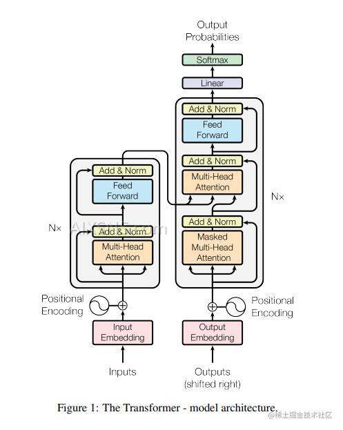
细看这个图，看不懂…直接逃跑了

原因，Transformer架构涉及到的前置知识点就有Self-Attention、Multi-Head Attention、Positional Encoding and so on.

下面将细细道来Transformer的前世今生。🚀

Embedding

由于Transformer最初出现时在nlp领域，之后才运用在图像等领域，所以在网络输入的之前，需要讲文本Embedding , 即向量化。

Embedding 是一个将离散变量转为连续向量表示的一个方式。

从网上找来一张图：

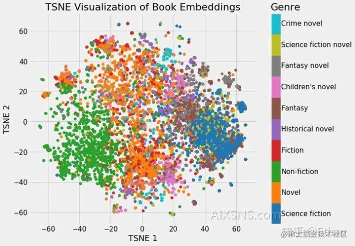
我们可以清楚地看到属于同一类型的书籍的分组。虽然它并不完美，但惊奇的是，我们只用 2 个数字就代表维基百科上的所有书籍，而在这些数字中仍能捕捉到不同类型之间的差异。这代表着 embedding 的价值。

在上图中，将书籍的Embedding结果可视化了。即每个点都代表一种书籍的分类。可以发现同一种类的书籍的Eemdding的结果是有聚类性质的，即同一类的聚合在某一块。

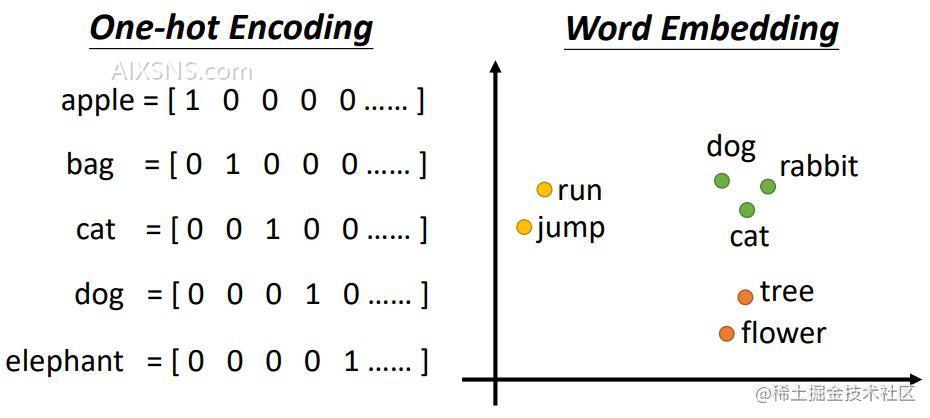
可能有朋友之前听过one-hot编码，那么one-hot编码和Eemdding又有什么区别呢？

one-hot编码是一系列的0，1 表示的比较长的向量。 但是Embedding却可以用(0.3,0.5)这种形式来表示一个物体。即使用低维(二维向量)表示一个高维的物体。

下图为两者Embedding的表示：

代码实现：

class Embeddings(nn.Module):
    def __init__(self, d_model, vocab):
        super(Embeddings, self).__init__()
        self.lut = nn.Embedding(vocab, d_model)
        self.d_model = d_model

    def forward(self, x):
        return self.lut(x) * math.sqrt(self.d_model)

Positional Embedding

接下来，要看的就是Positional Embedding了。

Positional Embedding 即 位置编码， 例如一句话： I like playing games.
games 这个单词和其他单词的位置信息肯定不相同，如果换成其他单词，词义也就变了。即在做机器翻译时，每个单词不仅需要考虑他本身的含义，还需要考虑这个单词在句子中的含义，甚至在整篇文章的作用。

在注解版的代码中，提到加入位置编码的原因：

Since our model contains no recurrence and no convolution, in order for the model to make use of the order of the sequence, we must inject some information about the relative or absolute position of the tokens in the sequence. To this end, we add “positional encodings” to the input embeddings at the bottoms of the encoder and decoder stacks.

翻译：由于我们的模型不包含递归和卷积，为了让模型利用序列的顺序，我们必须注入一些关于序列中标记的相对或绝对位置的信息。为此，我们在编码器和解码器堆栈底部的输入嵌入中添加“位置编码”。

Positional Embedding 在ViT模型中也出现过，下面这个图大家也一定很熟悉了

在上图中，由于需要将图片打成一个个的 Patch (批)， 但是将图片分割之后必然会损失一部分的信息，即在分割处的信息，所以我们可以加上 Positional Embedding —— 位置编码,

位置编码有很多种选择方式，在哈佛实验团队中的源码中使用的是sin 和 cos函数

$P{E}_{(pos,2i)}=\sin (pos/10000^{2i/d_{\text{model}}})$

$P{E}_{(pos,2i+1)}=\cos (pos/10000^{2i/d_{\text{model}}})$

选择sin和cos函数的原因：

We chose this function because we hypothesized it would
allow the model to easily learn to attend by relative positions,
since for any fixed offset $k$, $P{E}_{pos+k}$ can be represented as a
linear function of $P{E}_{pos}$.

翻译：对于任何固定偏移量$k$，$P{E}_{pos+k}$可以表示为线性的函数$P{E}_{pos}$。选择这个函数是假设它能通过相对位置轻松的学习到网络中的参数信息。

We chose the sinusoidal version because it may allow the model to extrapolate to sequence lengths longer than the ones encountered during training.

翻译：因为它可以允许模型外推到比训练期间遇到的序列长度更长的序列长度。

简而言之，就是方便网络更好的学习到对应的信息。

对应的实现代码

class PositionalEncoding(nn.Module):
    "Implement the PE function."

    def __init__(self, d_model, dropout, max_len=5000):
        super(PositionalEncoding, self).__init__()
        self.dropout = nn.Dropout(p=dropout)

        # Compute the positional encodings once in log space.
        pe = torch.zeros(max_len, d_model)
        position = torch.arange(0, max_len).unsqueeze(1)
        div_term = torch.exp(
            torch.arange(0, d_model, 2) * -(math.log(10000.0) / d_model)
        )
        pe[:, 0::2] = torch.sin(position * div_term)
        pe[:, 1::2] = torch.cos(position * div_term)
        pe = pe.unsqueeze(0)
        self.register_buffer("pe", pe)

    def forward(self, x):
        x = x + self.pe[:, : x.size(1)].requires_grad_(False)
        return self.dropout(x)

The positional encodings have the same dimension
$d_{\text{model}}$ as the embeddings, so that the two can be summed.

Positional Embedding 的大小和 输入的 Embedding 保持一致, $d_{\text{model}}$ 在文中是一个常量。

Self-Attention

经过Embedding之后，序列就要经过Multi-Head Attention,(多头自注意力)，介绍多头自注意力之前，必定得先介绍Self-Attention（自注意力）这个重要的机制了。

下面用到的图均来自李宏毅教授的PPT, 源地址 -> 李宏毅讲Self-Attention -> ppt课件

An attention function can be described as mapping a query and a set
of key-value pairs to an output, where the query, keys, values, and
output are all vectors. The output is computed as a weighted sum of
the values, where the weight assigned to each value is computed by a
compatibility function of the query with the corresponding key.

注意力函数可以描述为映射查询和集合输出的键值对，其中查询、键、值和输出都是向量。输出计算为值，其中分配给每个值的权重由查询与相应密钥的兼容性函数。

通过Self-Attention Layer层的序列长度保持一致，即输入的向量长度=向量长度

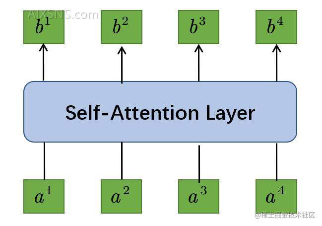
至于这中间的层的作用机理，请往下看：

所谓自注意力，也就是自己和自己的关联行为多大，向量和向量之间的关联有多大？

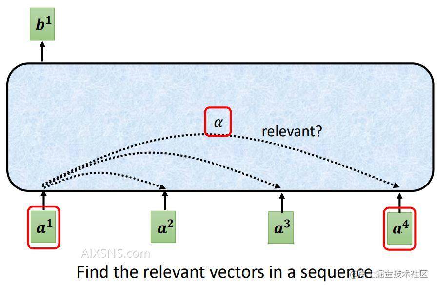
图/公式中的$a$ 为某一时刻的输入$x$乘以对应的权重矩阵。公式如下：

$a^i=W{x}^i$
($x$为某一时刻的输入序列)

那么如何计算自注意力的得分呢？如何判断哪两个向量的关联性更大呢？

Self-Attention论文中引入了Scaled Dot-Product Attention（缩放点积注意力），具体结构如下左图所示：

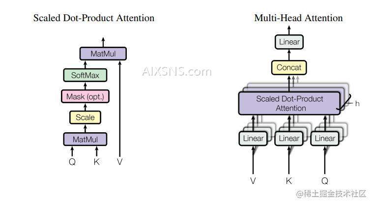
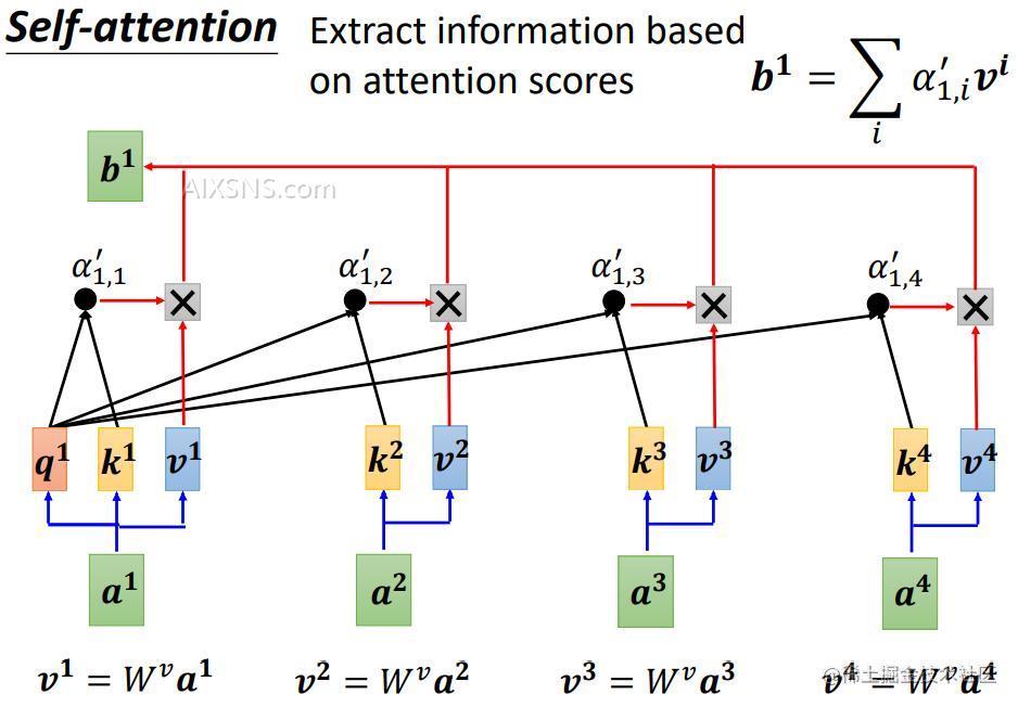
图中三个向量：$Q,K,V$, 就是Transformer图中的三个箭头。对应的公式为：

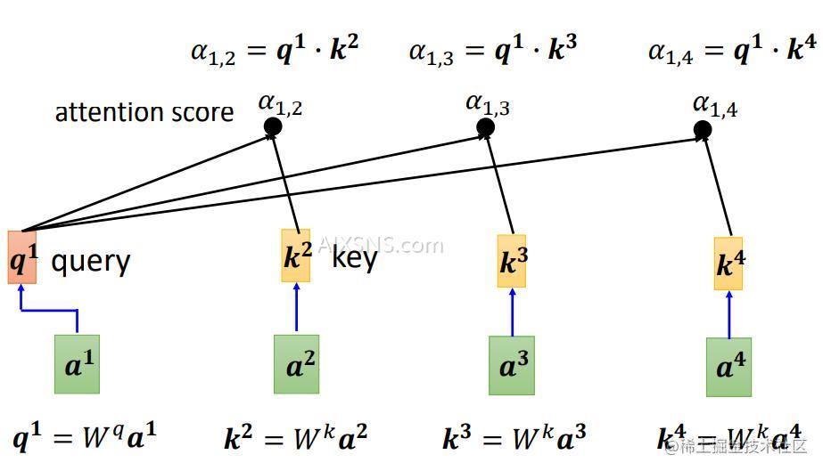
$q:query(tomatchothers):q^i=W^q{a}^i$

$k:key(tobematched)：k^i=W^k{a}^i$

$v:informationtobeextracted：v^i=W^v{a}^i$

$q$ 乘 $k$ 得到 $\alpha$ , 所以有
${\alpha }_{1,2}=q^1\cdot k^2{\alpha }_{1,3}=q^1\cdot k^2{\alpha }_{1,4}=q^1\cdot k^4$

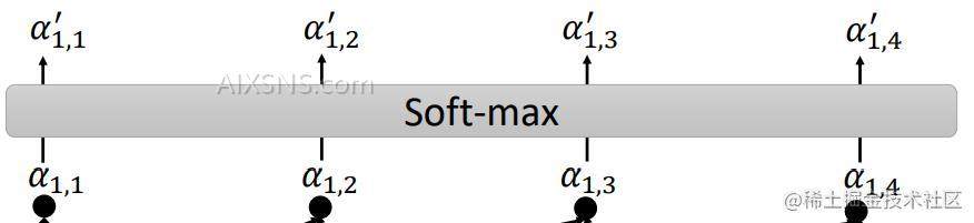
${\alpha }_{1,1}$ 通过 Softmax函数之后得到 ${\alpha }_{1,i}^{{}^{\prime }}$

Softmax计算公式为：
${\alpha }_{1,i}^{{}^{\prime }}=\frac{exp({\alpha }_{1,i})}{{\sum }_{j}exp({\alpha }_{1,j})}$

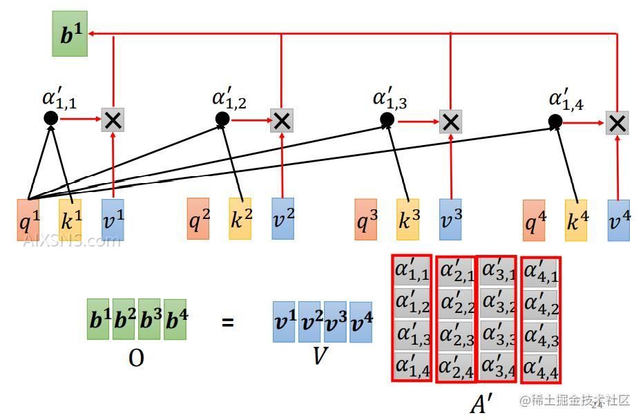
$\alpha$ 乘以 对应的 $v$ 并求和，即可得到对应的输出 $b$。 $b^1={\sum }_i{\alpha }_{1,i}^{{}^{\prime }}{v}^i$

$b^2$ 则是 $a^2$ 与其他向量计算注意力得分后的结果。

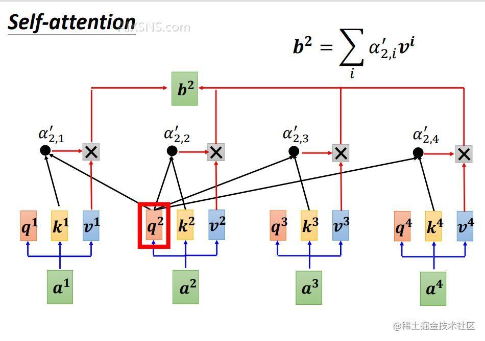
所以 $b^k$的计算公式为 $b^k={\sum }_i{\alpha }_{k,i}^{{}^{\prime }}{v}^i$

b 就是考虑了整个序列的输出 （vector considering the whole sequence）

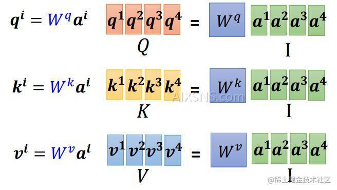
$Q,K,V$即对应的权重矩阵为对应的序列。$Q=[q_1,q_2,q_3,q_4]$

此时，我们再回顾一下Attention的计算公式，

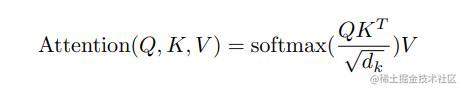
计 $Q{K}^T$ 计算的到的矩阵为$Attention$矩阵，简写为$A$， $A$矩阵经过Softmax并且除以${\sqrt{d}}_k$之后的矩阵计为$A^{{}^{\prime }}$。
具体计算图如下：

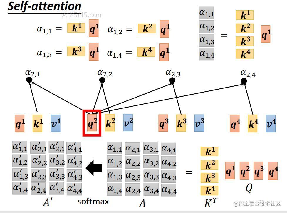
注意上图中没有标明除法，实际上计算是需要的。（为了防止计算量太大造成的额误差）这里为了画图方便，省去该步骤。

$A^{{}^{\prime }}$ 和 $V$ 作矩阵乘法，得到输出向量 $O=V\cdot A^{{}^{\prime }}=[b^1,b^2,b^3,b^3]$ 。

$W^q,W^k,W^v$ 是网络可学习的参数。

The two most commonly used attention functions are additive
attention (cite), and dot-product
(multiplicative) attention. Dot-product attention is identical to
our algorithm, except for the scaling factor of
$\frac{1}{\sqrt{d_k}}$. Additive attention computes the
compatibility function using a feed-forward network with a single
hidden layer. While the two are similar in theoretical complexity,
dot-product attention is much faster and more space-efficient in
practice, since it can be implemented using highly optimized matrix
multiplication code.

两个最常用的注意函数是加性的
和点积
（乘法）注意。点积注意与我们的算法，除了标定因子$\frac{1}{\sqrt{d_k}}$。加法注意计算
兼容性函数使用联邦学习网络与单个隐含层。虽然两者在理论复杂性上相似，点积的注意速度更快，空间效率更高实践，因为它可以使用高度优化的矩阵来实现乘法。

While for small values of $d_k$ the two mechanisms perform
similarly, additive attention outperforms dot product attention
without scaling for larger values of $d_k$
(cite). We suspect that for
large values of $d_k$, the dot products grow large in magnitude,
pushing the softmax function into regions where it has extremely
small gradients (To illustrate why the dot products get large,
assume that the components of $q$ and $k$ are independent random
variables with mean $0$ and variance $1$. Then their dot product,
$q\cdot k={\sum }_{i=1}^{d_k}{q}_i{k}_i$, has mean $0$ and variance
$d_k$.). To counteract this effect, we scale the dot products by
$\frac{1}{\sqrt{d_k}}$.

而对于$d_k$的小值，这两种机制执行同样，加性注意优于点积注意没有标定更大的价值$d_k$。
我们怀疑对于
$d_k$的大值，点积的大小变大，
将Softmax函数/最大化函数推送到小梯度（为了说明点积变大的原因，假设$q$和$k$的分量是独立随机的，均值为0、方差为1的变量。然后他们的点积，
$q\cdot k={\sum }_{i=1}^{d_k}{q}_i{k}_i$，均值为$0$、方差
为 $d_k$。）
为了抵消这种影响，我们将点积缩放为
$\frac{1}{\sqrt{d_k}}$。

如果不想关注到整个序列的信息，就需要引入掩码的概念，即将对应的矩阵权重置为0，这样在网络更新迭代中该部分就不会更新，仍然为0，从而达到目的。

Self-Attention计算有关的细节相信我已经描述清楚了 (水平有限，只能描述到这儿了，

代码实现如下：

def attention(query, key, value, mask=None, dropout=None):
    "Compute 'Scaled Dot Product Attention'"
    d_k = query.size(-1)
    scores = torch.matmul(query, key.transpose(-2, -1)) / math.sqrt(d_k)
    if mask is not None:
        scores = scores.masked_fill(mask == 0, -1e9)
    p_attn = scores.softmax(dim=-1)
    if dropout is not None:
        p_attn = dropout(p_attn)
    return torch.matmul(p_attn, value), p_attn

Multi-Head Atention

那么多头又是什么玩意儿呢？

在上面关于点积的图片，就出现了多头自注意力，，(不知视力好的你有没有发现呢？没错就是下面这张图

Multi-head attention allows the model to jointly attend to
information from different representation subspaces at different
positions. With a single attention head, averaging inhibits this.

多头注意力允许模型联合处理来自不同位置的不同表示子空间的信息。对于单个注意力头，平均抑制了这一点。

$$\begin{gathered} \mathrm{MultiHead}(Q,K,V)=\mathrm{Concat}(\mathrm{hea}{\mathrm{d}}_1,\dots ,\mathrm{hea}{\mathrm{d}}_{\mathrm{h}})W^O \\ \text{where}\mathrm{hea}{\mathrm{d}}_{\mathrm{i}}=\mathrm{Attention}(Q{W}_i^Q,K{W}_i^K,V{W}_i^V) \end{gathered}$$

Where the projections are parameter matrices $W_i^Q\in {\mathbb{R}}^{d_{\text{model}}\times d_k}$, $W_i^K\in {\mathbb{R}}^{d_{\text{model}}\times d_k}$, $W_i^V\in {\mathbb{R}}^{d_{\text{model}}\times d_v}$ and $W^O\in {\mathbb{R}}^{h{d}_v\times d_{\text{model}}}$.

In this work we employ $h=8$ parallel attention layers, or
heads. For each of these we use $d_k=d_v=d_{\text{model}}/h=64$. Due
to the reduced dimension of each head, the total computational cost
is similar to that of single-head attention with full
dimensionality.

在这项工作中，我们使用了h=8个平行的注意力层或头。对于其中的每一个，我们使用$d_k=64$ ,由于每个头的降维，总计算代价与全维度的单头注意力相近。

简而言之就是将一个头分散到多个头上，从而简化计算量。多头注意力的矩阵计算方式如下图：

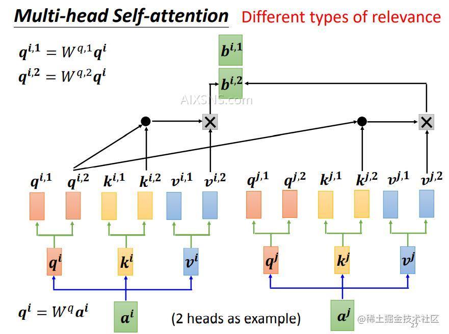
将一个$q$分解成$n$个q， 最后的输出即
$b^i=W^0[b^{i,1},b^{i,2}{]}^T$

代码实现如下：

class MultiHeadedAttention(nn.Module):
    def __init__(self, h, d_model, dropout=0.1):
        "Take in model size and number of heads."
        super(MultiHeadedAttention, self).__init__()
        assert d_model % h == 0
        # We assume d_v always equals d_k
        self.d_k = d_model // h
        self.h = h
        self.linears = clones(nn.Linear(d_model, d_model), 4)
        self.attn = None
        self.dropout = nn.Dropout(p=dropout)

    def forward(self, query, key, value, mask=None):
        "Implements Figure 2"
        if mask is not None:
            # Same mask applied to all h heads.
            mask = mask.unsqueeze(1)
        nbatches = query.size(0)

        # 1) Do all the linear projections in batch from d_model => h x d_k
        query, key, value = [
            lin(x).view(nbatches, -1, self.h, self.d_k).transpose(1, 2)
            for lin, x in zip(self.linears, (query, key, value))
        ]

        # 2) Apply attention on all the projected vectors in batch.
        x, self.attn = attention(
            query, key, value, mask=mask, dropout=self.dropout
        )

        # 3) "Concat" using a view and apply a final linear.
        x = (
            x.transpose(1, 2)
            .contiguous()
            .view(nbatches, -1, self.h * self.d_k)
        )
        del query
        del key
        del value
        return self.linears[-1](x)

k,v,q其实是一个东西，就是自己本身 但是后面乘以的$W$不同, 而$W$是网路中可学习的参数而已。

最后小结一下，本文主要讲述了Attention机制中的矩阵运算是如何实现的，以及在学习Attention结构中，出现的一些小细节。如为什么要除以${\sqrt{d}}_k$，为什么使用的点积而不是加法等进行阐述。

后续接着写完Transformer中的其他知识点。

这里十分感谢李宏毅教授的讲解以及哈佛团队的开源代码，在最前文的参考资料中已给出。如果不大清楚的可以去b站找找老师的视频讲解嗷~

如果对你帮助的话，不妨点个赞支持一下🚀~